Jobstreams Run Details - SLA Graph
The SLA Graph view of the Jobstream Run Details tab gives you an overview of the status of jobstream runs of one jobstream in relation to its SLA deadlines. In the view, a graphic plots the runs to reveal variances in run times and SLA deadline times at a glance, while a table provides numerous run statistics for filtering, sorting and comparing runs.
For a member of the operations team, this view of runs in relation to the SLA enables you to quickly assess the SLA compliance of a jobstream in recent runs as well as historically and how that affects predicted runs. If you are analyzing a jobstream's performance, you can view the SLA compliance for any filtered time range to discover patterns of compliance. Regardless of which process you are working in, when you identify a run of interest, you can drill down to the Gantt chart view in one click to see the job execution sequence and dependencies of the entire jobstream process.
The view is one of three views of jobstream run details, each of them show the same runs but presented differently to focus on another aspect of the run performance. You use them together to get insight into the performance issues of a jobstream. The other two are the following:
- Jobstreams Run Details - Actual
- Jobstreams Run Details - Relative to SLA, which also plots the run duration against the SLA deadline, but in a different way
You use these as part of your overall investigation of jobstream health and root cause research of runs that fail to meet their SLA deadlines. For more information, see Understanding the Jobstream Views.
This page includes the following:
Overview of the SLA Graph View of Jobstream Runs
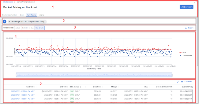
The SLA Graph view is one of three views on the Run Details tab for a jobstream. When the view is open, the page is comprised of several areas, as highlighted in the following graphic:
-
The page header contains the following:
-
A simplified breadcrumb path in the upper left corner that includes only Jobstreams > [Jobstream Name].
Click Jobstreams to close this jobstream and open the Jobstream Definitions page, which contains a list of all jobstreams. There you can select another jobstream to work with. For information, see Viewing Jobstream Definitions.
-
The name of the jobstream in large type, which is also the title of the page
-
The Edit Jobstream button that opens the jobstream definition for editing. For information, see Adding and Editing Jobstreams.
-
Tabs to switch to the various jobstream details tab pages. For information, see Viewing Jobstream Definitions.
-
-
The filter toolbar allows you to filter the list in this view and shows you which filters have been applied to the list. You can filter the list of jobstream runs by date range and final run status (early, late, unknown, and so on). The default filter is only for the time range. It is set to show the runs of only the last 7 days to the next 1 day. For more information, see Using Filters (Web Interface).
Note:When you filter on status, the list that opens offers only the statuses that are relevant to the runs in the filtered time range.
-
The Time Source toolbar contains various controls to change what you are viewing:
-
Click the Time Source buttons to switch among the three Run Details views: Actual, Relative to SLA, and SLA Graph. The view that you are on is highlighted.
-
Click the Export button to export the tabular data in the view, as you see it, to a CSV file, which lands in your Downloads folder. The file contains the filtered data as they are arranged and sorted in the columns in your view. For more information, see Exporting Table Data.
-
-
The SLA Graph in the top part of the page. This can be a scatter diagram for end-time SLAs and a candlestick diagram for duration-based SLAs. For a full description, see The SLA Charts for Each SLA Type below.
-
The table of jobstream runs in the bottom part of the page. For a full description, see The Table of Jobstream Runs below.
The SLA Charts for Each SLA Type
The upper part of the SLA Chart view contains the chart. Depending on whether the SLA defined for the jobstream is an end-time SLA or a duration SLA, you see a different type graph.
Common Characteristics
Regardless of the SLA type, the following is always true about the chart:
- The x-axis measures the Start Date/Time of the runs.
- The y-axis measures the jobstream run time, whether it is a Time of Day for end-time SLAs or a Duration time.
- Color-coded dots mark start/end times and durations of a run.
- Blue dots mean that the SLA deadline was met.
- Red dots mean that the SLA deadline was exceeded.
- The red dotted line across the graph shows the SLA deadline.
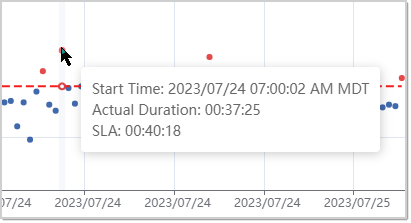
- When you point to a specific run on the SLA line, a red circle appears for the SLA deadline.
- When you mouseover any data point, a tooltip that shows run details appears. For runtime SLAs the details include the start time, the actual duration, and the SLA duration. For duration SLAs, the details include the start time, end time, and SLA.
- You can click a data point for a run to open the Gantt chart view for the run. For more information, see The Gantt View for a Jobstream Run (Web Interface).
- You can zoom in and out on the graph in one of two ways:
- By rolling your mouse wheel up and down. Use this to zoom in and out equally from both sides of the time span around the date and time that you have positioned your mouse pointer when you roll the wheel.
- By clicking and dragging the handles to the point in time you want to include. Use this when you want to choose a time span that is not a symmetrically zoom within the filtered time span.
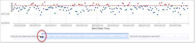
Note that, although you can zoom out, you cannot exceed the date range set in the filter for the tab page. Furthermore, zooming in and out on the graph has no affect on which jobstream runs are included on the table below it. The content in the table is controlled by the filters.
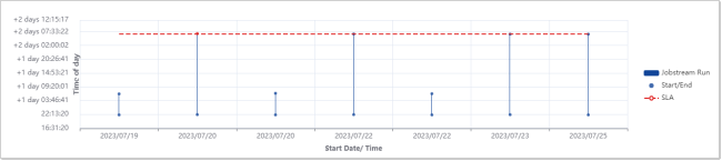
Graph for Time-based SLAs
For jobstreams with a time-based SLA, the y-axis shows times of day. On these graphs you see a candlestick representation of each run, showing a vertical line spanning the start to the end time. For the corresponding SLA, you see a red dot in the same vertical axis for the point in time by which the run must end to meet the SLA deadline. For this reason, typically, the SLA points are all on the same horizontal line. For jobstreams with a system-calculated, time-based SLA, the line might not be straight because the deadline might start to vary as the system adjusts its calculations based on a growing set of run history data.
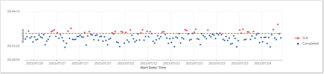
Graph for Duration-based SLAs
For jobstreams with duration-based SLAs, the y-axis measures a time span, rather than a time of day. Because jobstream runs can begin at different times, you just see a dot for the final time of the run. Blue dots for the end times of runs that ended within the prescribed duration. Red dots for the end times of runs that exceeded the defined duration limit. The SLA end times are plotted along a red dotted line. When you mouseover the dotted SLA line in the same vertical axis as the dot for the end time of a run, an empty red circle appears to indicate the SLA time for that run.
The Table of Jobstream Runs
The table of jobstream runs in the bottom part of the SLA Chart view of the Run Details tab lists the completed, currently running, and predicted runs for the jobstream within the filtered date range and run statuses.
For each run, the following jobstream run statistics are available in the data columns.
-
Start Time
When the jobstream run started. This is the start time of the first job in the jobstream. This is also a link that you can click to open the Gantt chart view for the run. For more information, see The Gantt View for a Jobstream Run (Web Interface).
-
End Time
When the jobstream run completed. This is the end time of the last job in the jobstream.
-
SLA Status
For an in-progress jobstream run, this is the current run status of the jobstream. For a completed jobstream run, this is the final status of the jobstream run. It indicates whether the jobstream completed in time to fulfill the SLA criterion (EARLY) or failed to do so (LATE).
-
Duration
The length of time that the jobstream ran from start to finish.
-
Margin
The margin is the deviation of the duration of this jobstream run from the absolute average of the durations of all runs of this jobstream that AAI has stored in its historical database.
-
Jobs In Critical Path
The number of jobs in a jobstream that are on the critical path for a particular run. This can vary for different runs of the same jobstream, depending on run conditions, jobs dependencies, and which branch of processing might be triggered based on data and conditions for the run.
-
Overall Delay
The sum time of all the delays for a jobstream run.
-
Start-to-Running Delay
The difference between the Start Time and the Running Time for the jobstream. This indicates the time that the scheduler takes to prepare resources to run the first job. High start-to-running delays can point to scheduler inefficiencies or suboptimal load distribution.
The start-to-running delay of a job is included in the System Delay for the jobstream as a whole.
-
Finish-to-Start Delay
A sum of all the finish-to-start delays for the jobs in the jobstream. A finish-to-start delay for a job is the time that passed after the job's last predecessor finished and before the job started. High finish-to-start delays indicate scheduler inefficiencies because there is too much wait time that could be used in processing time. You might want to redistribute the workload on your agents.
The finish-to-start delays of the jobs in the jobstream run are is included in the System Delay for the jobstream as a whole.
Be aware that the time when a job is on-hold is included in finish-to-start delay, not operational delay.
-
System Delay
This is the sum of the start-to-running and the finish-to-start delays of all the jobs within the jobstream run. When these delays are high, this is an indication that you should look at where you can optimize your scheduler workloads.
-
Design Delay
This is any delay that is hard-coded into the schedule, such as a hard-coded start time.
Tip:Although there might be exceptions, defining hard-coded job start times is not recommendable in a production environment because they can lead to inefficient gaps in processing time. Furthermore, some time after the job is originally defined, this kind of hard-coding can lead to semantic errors in your job processes. Problems like a reference to a deprecated calendar, a deleted job, or other missing object that can go undetected.
Rather than specifying hard start times, you should define start times based on direct dependencies on predecessors.
-
Operational Delay
This is the amount of time between when a jobstream failed and started running again. It reflects how long an operation teams take to fix an issue.
Refreshing the table data
Use the Refresh Datagrid button, which you find above the table to the right, to immediately bring up the latest data from the AAI database, rather than wait for the next automatic refresh (30 seconds by default). The last time at which data was fetched, whether automatically or because you clicked this button, appears to the left of the button.
Filtering and organizing the table data
By using a combination of filters and table configuration options, you can extract and organize the run data in a meaningful way. This is helpful while working with the SLA Graph view online. It is also important when exporting the jobstream run data because the exported file will contain only the filtered data and in the way the table is configured.
All the AAI table configuration features are available to the table on the SLA Graph view. These include the following:
- Selecting table columns to show or hide from the Columns menu.
- Sorting the table according to the values in any column by clicking column headers.
- Using drag-and-drop to move columns to put data columns that you want to compare next to each other. When you are viewing the table online, you can move essential data columns to the left where you can see them without having to scroll horizontally.
For more information, see Working with Tables (Web Interface).
See also: